If you’re at all interested in procedural generation, digital art or game development, it’s very likely that you’ve heard about the wave function collapse (WFC) algorithm before. It’s incredible popular, has been ported to virtually every language and engine, and used in several games.
In essence, WFC is a texture synthesis algorithm that generates an output image with a desired size that is as similar as possible to a given sample image. WFC tries to ensure local similarity, meaning that the output image can only contain NxN patterns of pixels that are prersent in the input.
The following example (taken from the best known WFC repo) shows an example of the technique. The given image is on the left, with the generated output on the right. N = 3 here, so every 3x3 tile in the output can be found in the input.
A Little bit of Formalization
The name “wave function collapse” sounds cool and refers to a quantum mechanics, but the technique is actually very simple.
Many sources make an explicit distinction between the so called “overlapping” and “tiled” mode of WFC. For example, this and this page do a good job of explaining the latter, but both techniques can in fact be cleanly expressed in the same general framework.
Let T be a set of tiles (small sprites) with dimensions w x h. The goal is to fill up a grid so that each cell contains exactly one tile. In the initial state, each tile is possible at every cell so that: G[x][y] = T for each x, y. The user also needs to define a neighborhood function N: ℕxℕ ↦ P(ℕxℕ). In most cases, this is simply the von Neumann neighborhood (or 4-neighborhood) so that N(x,y) = {(x-1,y), (x+1,y), (x,y-1), (x,y+1)} (without crossing the grid boundaries, but setups where the grid wraps around are also sometimes used).
For the sake of notation, it is perhaps easier to define a set of named offsets instead, e.g. O = {L: (-1, 0), R: (1, 0), U: (0, 1), D: (0, -1)} and write something like neighbor(L, 1, 3) (coordinates for cell on the left of the one at x=1, y=3). The exact definitions are trivial but verbose so omitted here.
Finally, the user provides a set of constraints C which states which tiles are allowed to be a neighbor of others for the different offsets. (Constraints expressing which tiles are not allowed is also possible; it doesn’t change the setup, but the former makes the algorithm below read a bit easer.)
The algorithm itself then works as follows:
while there still cells with more than one tile:
    min_val = min({∀ x, y : |G[x][y]| | |G[x][y]| > 1 })
    min_cells = {∀ x, y: (x,y) | |G[x][y]| = min_val }
    cell_to_collapse = random(min_cells)
    tile_to_use = random(G[cell_to_collapse])
    G[cell_to_collapse] = {tile_to_use}
    propagate(cell_to_collapse)
In short, as long as there are still cells to “collapse” (i.e. decide their tile), pick a random cell out of the set which allows for the least amount of choices and pick a random valid tile for it. This follows a minimum entropy heuristic and is similar how to humans perform search. This procedure is not guaranteed to end in a state where all tiles can be collapsed and so some restarts might be required, but in most cases (with a generous set of tiles and constraints), it works well enough.
The propagate function starts from the x, y coordinates of the cell we have just “collapsed” and updates the neighboring cells based on this new information we have obtained. That is, we can take out potential tile choices from surrounding cells as we know based on the constraints they will not be valid any longer, i.e.:
# Wrong version of propagate
propagate(x, y):
    for offset in O:
        neighbor_coords = neighbor(offset, x, y)
        G[neighbor_coords] = {∀ t in T : t | allowed(offset, x, y, t)}

allowed(offset, x, y, candidate_tile):
    neighbor_coords = neighbor(offset, x, y)
    # Is there a tile in the "center" cell
    # which is compatible with the candidate tile?
    return ∃ ∀ ct in G[x][y] : (offset, ct, candidate_tile) ∈ C
Why is this wrong? Because this fails to take into account that if we change the set of possible tiles for a cell based on the one we just collapsed, that information, too, should be propagated to its neighbors. So we need to keep track of a stack instead:
# Correct version of propagate
propagate(x, y):
    to_do = {(x, y)}
    while |to_do|:
        x, y = pop(to_do)
        for offset in O:
            neighbor_coords = neighbor(offset, x, y)
            len_before = |G[neighbor_coords]|
            G[neighbor_coords] = {∀ t in T : t | allowed(offset, x, y, t)}
            if |G[neighbor_coords]| != len_before:
                to_do += {neighbor_coords}
That’s all there is to it.
Small Example
This is enough to understand what most resources refer to as the “tiled” mode of WFC. For example, say that we have T = {mountain, grass, beach, water} and C = {(L, water, water), (L, water, beach), (L, beach, water), (L, beach, beach), (L, beach, grass), (L, grass, beach), (L, grass, grass), (L, grass, mountain), (L, mountain, grass), (L, mountain, mountain), … (repeat for the other offsets)}. In other words, we have a simplistic and symmetric set of allowances here where water can be next to water or beach, a beach can be next to water, beach or grass, and so on.
The tiles themselves are just visualized in a solid color, and running the algorithm then gives the following result:
Moving to the Overlapping Mode
Once you understand the above, it is very easy to make the jump to the so called “overlapping” mode. Let’s try this out with the typical “flowers” example:
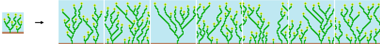
The set of tiles T here is simply extracted by sliding a window with dimensions w x h over the input image:
Typically, a 2x2 or 3x3 pattern is used to do so.
The set of allowances C is then simply based on whether to tiles where next to each other somewhere in the given input image for the given (offset) direction.
The final “trick” to understand is that to visualize our grid G, we need to overlap the tiles again with each other (each tile needs to move w-1 to the left and h-1 upwards).
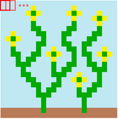
And then we get the following end result for a 2x2 set of tiles:
If we try this with one of the 3x3 examples, however, we might find that it does not work as expected:
The “mistake” made here is that we didn’t allow sliding window to go outside the boundaries of the template image and wrap around. Once we fix that, we get the expected result (the grayscale color used here indicates the number of possibilities left for non-collapsed cells):
More Tiles
A final gotcha to be aware of when working in overlapping mode especially is the fact that in most cases, we do not only want the sliding window to go outside the boundaries of the template image, but we also want to create additional tiles from each of the ones we extract by rotating them, or flipping them along the horizontal and/or vertical axis.
When this is done, one however needs to be careful when constructing the set of allowance constraints as we can’t simply do so by matching tiles with the input image. Hence, the set of allowances should be constructed dynamically by iterating over each pair of tiles, iterating over all the offsets, and checking whether the pixel colors match. In other words, whether the pair of tiles overlaps according to the given offset.
This website allows you to play around with a fast implementation of the overlapping mode and lets you draw your own pattern as well. I’m embedding it below so you can play around with it:
Supervised WFC?
Continuing from this basic setup, a lot of people have been working to create more constrained versions of WFC, typically by coming up with methods to also make the technique globally constrained. A simple example would be to insure for instance in our first example that there is a walkable path of grassland from, say, top to bottom. Such global constraints are typically necessary when applying WFC in games.
There are different approaches to tacke this. Perhaps the easiest would just be to continue restarting the algorithm until a solution is found which satisfies the global constraints. Another one is to tackle the global constraints by post-processing the generated image (and accept the fact that the image might not be fully locally consistent any longer). Other approaches implement a form of backtracking and checking inside of the WFC algorithm itself. The Caves of Qud developer has a good talk on this, and so does the dev of Bad North.
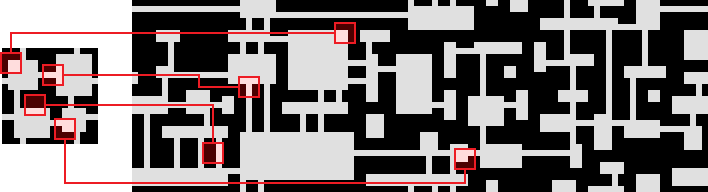
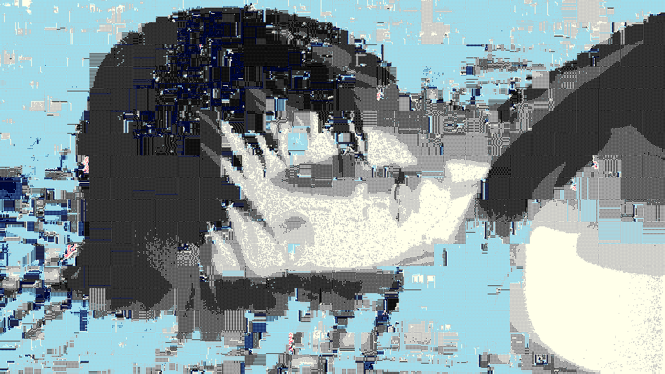
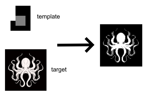
Something which I have been exploring a while ago whilst looking through loackme’s work was whether WFC would also lend itself to creating this kind of glitch art. Starting from a target image, instead of using tile_to_use = random(G[cell_to_collapse]), I instead picked the tile which pattern was closest to the corresponding spot in the target image. I first used RMSE to do so but later switched to using the Euclidean distance between two points in Lab color space instead, which worked a lot better.
Since my implementation was very slow, I perform the generation in a multi-threaded way by just slicing up the image into smaller squares and running WFC on each of them. This breaks the local constraints at the edges of the smaller squares, which can be mitigated if you’re careful how you go over the squares (i.e. with the neighborhood above, a checkerboard pattern would work), but I found it makes the results look interesting as well.
Depending on the template used, you can pretty good or at least diverse results this way:
WFC as Constraint Programming
Whilst playing around with this, I also realized you could probably implement WFC as a constraint programming problem. I was heavily using CP-SAT for a serious project at the time. I got quite excited about the possibility to potentially write a short conference paper on this, but Isaac and Adam at the University of California Santa Cruz already beat me to it in 2017.
Oh well, they implement it using Choco, so we can at least have a bit of programming exercise using CP-SAT.
A basic implementation boils down to this:
from ortools.sat.python import cp_model
from random import randint

OFFSETS = {
    "up": (0, -1),
    "dn": (0, +1),
    "le": (-1, 0),
    "ri": (+1, 0),
}

RULES = { # My <dir> neighbor can be any of this
    "━": {"up": '━┗┛ ', "dn": '━┏┓ ', "le": '━┏┗', "ri": '━┛┓'},
    "┃": {"up": '┃┏┓', "dn": '┃┗┛', "le": '┃┛┓ ', "ri": '┃┏┗ '},
    "┏": {"up": '━┗┛ ', "dn": '┃┗┛', "le": '┃┛┓ ', "ri": '┛┓━'},
    "┓": {"up": '━┗┛ ', "dn": '┃┗┛', "le": '━┏┗', "ri": '┃┏┗ '},
    "┗": {"up": '┃┏┓', "dn": '━┏┓ ', "le": '┃┛┓ ', "ri": '━┛┓'},
    "┛": {"up": '┃┏┓ ', "dn": '━┏┓ ', "le": '━┏┗', "ri": '┃┏┗ '},
    " ": {"up": '━┗┛ ', "dn": '━┏┓ ', "le": '━┛┓ ', "ri": '━┏┗ '},
}

TILES = list(RULES.keys())

GRID_SIZE = (40, 10)

model = cp_model.CpModel()
position_to_tiles = {}
tiles_to_amount = {}

# Exactly one tile per cell
for x in range(GRID_SIZE[0]):
    for y in range(GRID_SIZE[1]):
        position_to_tiles[(x, y)] = [
            model.NewBoolVar(f"position_to_tile_{x}_{y}_{i}") \
                for i in range(len(TILES))
        ]
        model.Add(sum(position_to_tiles[(x, y)]) == 1)

# Ensure local consistency
for x in range(GRID_SIZE[0]):
    for y in range(GRID_SIZE[1]):
        pos = (x, y)
        c_var = position_to_tiles[pos]
        for offset_key, offset in OFFSETS.items():
            n_pos = (x + offset[0], y + offset[1])
            if n_pos[0] < 0 or n_pos[1] < 0 or n_pos[0] >= GRID_SIZE[0] or n_pos[1] >= GRID_SIZE[1]:
                continue
            for t in range(len(TILES)):
                allowable_bools = [
                    position_to_tiles[n_pos][TILES.index(allowed)] \
                        for allowed in RULES[TILES[t]][offset_key]
                ]
                model.Add(sum(allowable_bools) >= 1).OnlyEnforceIf(c_var[t])

def pr_sol(sol, position_to_tiles):
    for y in range(GRID_SIZE[1]):
        for x in range(GRID_SIZE[0]):
            for t in range(len(TILES)):
                if sol.Value(position_to_tiles[(x, y)][t]) > 0:
                    print(TILES[t], end="")
        print("")
    print(""); print(""); print("")

solver = cp_model.CpSolver()
solver.parameters.random_seed = randint(0, 10000)
solver.parameters.log_search_progress = True

result = solver.Solve(model)
pr_sol(solver, position_to_tiles)
A random seed is set to generate a different solution every time. When we run this, we see:
┓┏┛ ┏┓┃┗┓┃┃┏━┓┃┃┃┏━━┛ ┏━┛┗┛ ┗┛┗┛ ┗━━━━┓┗
┛┗┓ ┗┛┃┏┛┃┗┛ ┗┛┗┛┗┓┏┓┏┛┏┓   ┏┓┏━┓┏┓┏┓ ┗┓
━━┛┏━┓┃┗┓┗━┓┏┓┏━━━┛┗┛┗┓┃┗━┓ ┗┛┗┓┃┃┗┛┗━━┛
┏━┓┃┏┛┗━┛ ┏┛┃┗┛ ┏┓  ┏┓┗┛  ┗━━━━┛┃┗┓┏━━┓┏
┗┓┃┃┃┏┓┏━━┛ ┗━┓ ┗┛┏┓┃┃┏┓┏━┓  ┏┓ ┗┓┃┃┏━┛┗
┓┃┃┃┃┃┗┛┏━┓┏┓ ┗┓┏┓┃┃┗┛┃┗┛ ┗━━┛┃┏━┛┃┗┛┏━━
┛┗┛┃┗┛  ┗┓┃┃┗┓┏┛┗┛┗┛┏━┛┏━━━━┓ ┗┛  ┗┓┏┛
┓  ┗━━┓  ┗┛┗┓┃┃┏┓ ┏┓┗━━┛┏━━━┛ ┏━━━━┛┗━┓
┛   ┏━┛ ┏┓┏━┛┃┃┃┗━┛┗┓┏━┓┃┏━━┓┏┛ ┏━━━┓ ┗━
┏━━┓┗━┓ ┗┛┃┏━┛┃┃┏┓┏━┛┗━┛┗┛┏┓┗┛  ┗━┓ ┗┓┏┓
A benefit of this is that this setup lends itself extremely well to adding additional constraints. For instance, we can easily add a constraint that states that at least 200 cells must be spaces:
# At least 200 cells must be spaces
model.Add(sum(position_to_tiles[(x, y)][TILES.index(" ")] \
              for x in range(GRID_SIZE[0]) for y in range(GRID_SIZE[1])) >= 200)
Which looks like this:
 ┗┛    ┏┓  ┏┛ ┏┛┃┗┛ ┗┓  ┗┛┃┗┛┏┓      ┗━━
       ┗┛  ┗━┓┃┏┛  ┏━┛  ┏━┛  ┗┛
     ┏┓    ┏━┛┗┛   ┗┓   ┗━━━┓┏┓      ┏━━
     ┗┛┏┓ ┏┛        ┗━┓   ┏┓┃┃┗┓     ┗┓
  ┏━━━┓┃┗━┛        ┏━┓┗━━━┛┃┃┃┏┛   ┏┓ ┗━
  ┗┓ ┏┛┗━┓         ┗━┛     ┗┛┗┛ ┏┓ ┗┛
  ┏┛┏┛   ┗┓   ┏┓          ┏┓  ┏━┛┃┏━━┓
┓┏┛┏┛     ┗━┓ ┗┛      ┏━┓ ┗┛ ┏┛  ┗┛ ┏┛ ┏
┗┛ ┗┓       ┗┓  ┏┓  ┏┓┃┏┛  ┏┓┗┓     ┗━━┛
   ┏┛       ┏┛ ┏┛┗━┓┗┛┗┛   ┗┛ ┗━┓
What we can also easily do since we’re using CP-SAT is add an objective. E.g. to ensure we get enough variation, we could maximize the entropy of the generated pattern using something like Σ -sum(p * log(p)) for each cell with p being the number of times the tile appears in the map divided by the map size. The issue is that this is difficult to implement in CP-SAT.
An easier proxy is to minimize the difference between the maximum and minimum times a tile appears:
# Attempt to maximize entropy: minimize max(t) - min(t)
t_counts = []
for t in range(len(TILES)):
    t_counts.append(model.NewIntVar(0, GRID_SIZE[0]*GRID_SIZE[1], f"weight_of_{t}"))
    model.Add(t_counts[-1] == sum([
        position_to_tiles[(x, y)][t]
        for x in range(GRID_SIZE[0])
        for y in range(GRID_SIZE[1])
    ]))
max_t = model.NewIntVar(0, GRID_SIZE[0]*GRID_SIZE[1], f"max_t")
min_t = model.NewIntVar(0, GRID_SIZE[0]*GRID_SIZE[1], f"min_t")
model.AddMaxEquality(max_t, t_counts)
model.AddMinEquality(min_t, t_counts)

model.Minimize(max_t - min_t)
This provides us with this:
 ┏┛┗━┛       ┗┛    ┏┓┃┗┓┗━┛┗┓┃┃┃┏┓┃┏┛┗┓
━┛                 ┗┛┗┓┃┏┓┏━┛┃┃┃┗┛┃┗━━┛
                    ┏━┛┗┛┗┛┏┓┃┃┗━┓┃┏━━━┓
                    ┗━━┓ ┏━┛┃┗┛┏┓┗┛┗━━┓┗
                       ┗━┛┏━┛┏┓┃┗━┓   ┗┓
                     ┏━┓┏┓┗━┓┃┃┃┏━┛ ┏━┓┃
                     ┗┓┗┛┃┏━┛┃┃┃┗━┓┏┛ ┗┛
                    ┏┓┗━━┛┃┏┓┗┛┃┏━┛┃┏┓┏━
                   ┏┛┗━━━┓┗┛┃┏┓┃┗━┓┃┗┛┃┏
    ┏┓             ┗┓┏┓ ┏┛ ┏┛┗┛┃┏┓┃┗┓┏┛┃
Though this is still a bit imbalanced topology-wise. Perhaps we can do better by looking at repetitions of NxN patterns instead? This is quite a challenge to express as an objective. Perhaps we can take a different approach: what we want to avoid is having that large areas filled with space on the left, so lets tackle that. One obvious way would just be to say that for any NxN area, we disallow that area from being filled up with space:
# Avoid large space
N_size = 3
for x in range(GRID_SIZE[0]-N_size):
    for y in range(GRID_SIZE[1]-N_size):
        model.Add(sum(
            position_to_tiles[(xp, yp)][TILES.index(" ")] \
                for xp in range(x, x+N_size) for yp in range(y, y+N_size)
            ) < N_size**2)
That seems to work pretty well:
       ┏┛                ┏┛       ┗┓
       ┗┓┏┓       ┏━━┓ ┏━┛       ┏┓┗┓  ┏
 ┏━━━━━┓┃┃┃┏━━━┓┏┓┗━━┛ ┗━┓  ┏━┓  ┗┛ ┗━━┛
┏┛  ┏┓ ┗┛┃┃┗┓  ┗┛┗┓    ┏┓┗━━┛┏┛
┛   ┗┛  ┏┛┗━┛    ┏┛  ┏┓┃┃┏┓  ┗┓   ┏┓ ┏┓┏
       ┏┛     ┏━┓┃┏━┓┃┃┃┃┗┛   ┗━━┓┃┗┓┃┃┃
  ┏┓ ┏━┛  ┏┓  ┗━┛┃┗┓┃┃┃┃┃┏━┓    ┏┛┗┓┃┃┃┃
━┓┃┃┏┛    ┗┛     ┗━┛┃┃┃┃┗┛┏┛    ┗━┓┃┗┛┗┛
 ┗┛┗┛               ┗┛┗┛  ┗━━━┓   ┗┛
                              ┗┓    ┏┓
(We could in fact add the same constraint for all of the tiles. An extension could also entail checking this for sizes from NHigh to NLow and then including minimization of the size in the objective.)
We can also try to generate a space filling curve. We can do so by first creating a Hamiltonian cycle over the cells and then maximize the length of the cycle in the objective. We keep in the previous constraints to make it challenging.
# Construct Hamiltonian cycle
arcs = []
pos_to_nr = {}
nr_to_pos = {}
pos_nr = 0
for x in range(GRID_SIZE[0]):
    for y in range(GRID_SIZE[1]):
        pos_to_nr[(x,y)] = pos_nr
        nr_to_pos[pos_nr] = (x,y)
        pos_nr += 1

for x in range(GRID_SIZE[0]):
    for y in range(GRID_SIZE[1]):
        pos = (x, y)
        c_var = position_to_tiles[pos]
        self_lit = model.new_bool_var(f"self_lit_{x}_{y}")
        arcs.append((pos_to_nr[pos], pos_to_nr[pos], self_lit))
        for offset_key, offset in OFFSETS.items():
            n_pos = (x + offset[0], y + offset[1])
            if n_pos[0] < 0 or n_pos[1] < 0 or n_pos[0] >= GRID_SIZE[0] or n_pos[1] >= GRID_SIZE[1]:
                continue
            lit = model.new_bool_var(f"lit_{x}_{y}_{n_pos[0]}_{n_pos[1]}")
            for t in range(len(TILES)):
                if " " in RULES[TILES[t]][offset_key]:
                    model.Add(lit == 0).OnlyEnforceIf(c_var[t])
            arcs.append((pos_to_nr[pos], pos_to_nr[n_pos], lit))

model.add_circuit(arcs)

# Change the objective:
model.Maximize(sum([a[2] for a in arcs if a[0] != a[1]]))
This is actually a hard task given that the underlying graph is pretty large but after half an hour we get an optimal solution:
┏┓
┃┗━━━━━━━━━━━━━━━━━━━━━━━━━━━━━━━━━━━┓
┃┏━┓                     ┏━━┓    ┏━━━┛
┃┗┓┗┓            ┏━┓  ┏━┓┗┓ ┗┓┏┓ ┗━━┓
┗┓┗┓┗━┓  ┏━━━┓  ┏┛ ┗┓┏┛ ┗┓┗┓ ┗┛┗━━━┓┗┓
 ┗━┛  ┗┓ ┗┓  ┗┓ ┗━━┓┗┛   ┗┓┗━━━━━━┓┗┓┗━┓
       ┗┓ ┗┓  ┗┓   ┗━━━┓  ┗┓      ┗┓┃┏━┛
        ┗┓ ┗━┓ ┗┓  ┏━━┓┗━┓ ┗━━━━━━┓┃┃┗━┓
         ┗━━━┛  ┗━━┛  ┗━━┛        ┗┛┗━━┛
Supervised Generation with CP
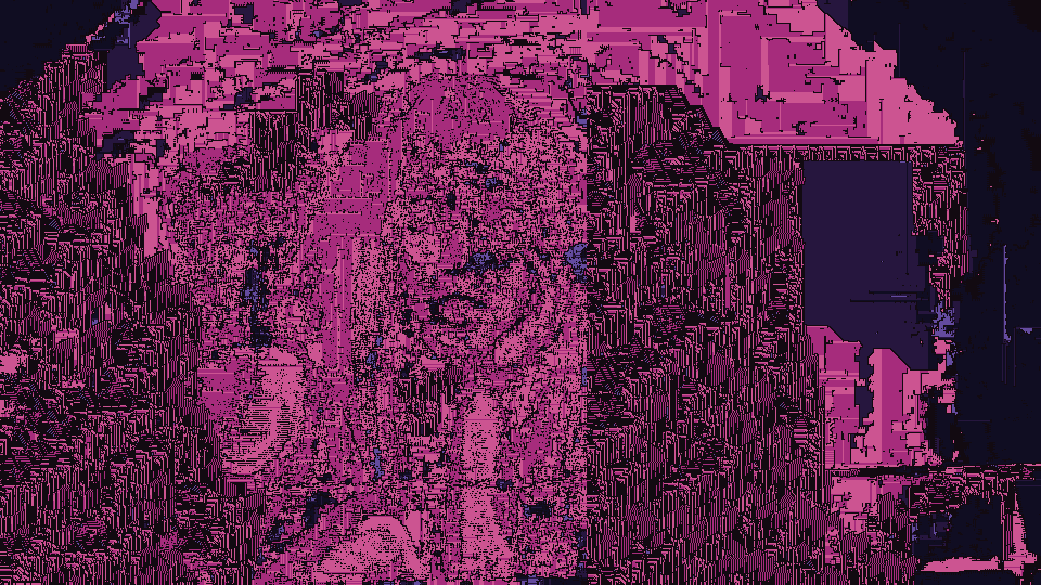
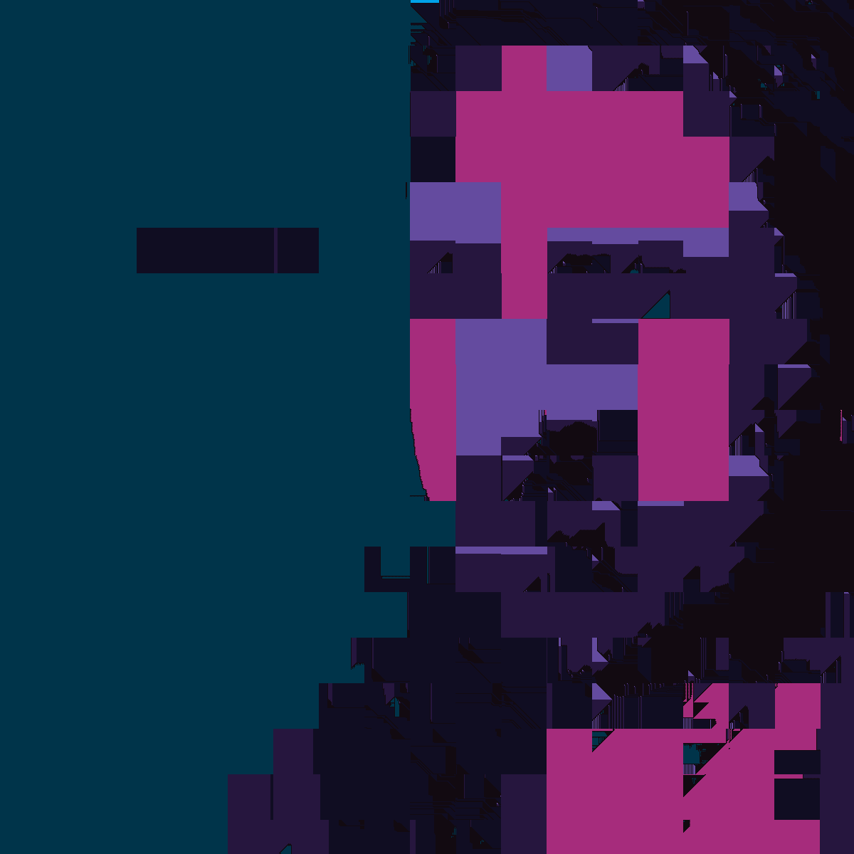
Finally, we can attempt to convert the “supervised generation to look similar to a given image” approach to work within the CP framework. The basic setup is not even that difficult as for each possible tile and each possible location, we can pre-calculate what the similarity between them is, and then just maximize the similarity over the whole map.
For relatively small images, CP-SAT is actually quite capable at this, as seen in the following example:
This solution is very close to its bound, but proving optimality does take a very long time. Nevertheless, a good-enough solution is reached after 10 minutes. Even though it’s similarity to the target image is less, it is correct in terms of WFC constraints and the additional glitchiness makes it look good as well:

What’s even cooler is that we can keep track of the different solutions as they are being produced (each with a better similarity to the target image), stick them in a GIF, and show them.