In 2019, I wrote on the topic of discovering which features interact in a model agnostic manner, using an approach from a paper by Friedman and Popescu entitled Predictive Learning Via Rule Ensembles. I wanted to revisit the topic briefly and expand on it somewhat, given that scikit-learn has progressed a bit since then.

On Permutation Feature Importance, Partial Dependence, and Individual Conditional Expectation Plots

First the good news: scikit-learn has added support both for permutation based feature importance (and should now be your go-to approach instead of the feature_importances_ attribute) as well as support for partial dependence plots. ICE plots are also supported in the latest version through the kind parameter.

Since plot_partial_dependence supports two-way interactions as well, this by itself already removes having to depend on lots of other libraries (though I still recommend rfpimp, if only for their more explicit handling of feature correlation).

Revisiting Friedman’s H-statistic

Recall that we had defined two versions of the H-statistic in the previous post:

• H2(jk) to measure whether features j and k interact. For this, partial dependence results need to be calculated for j and k separately, and j and k together. The second-order measure
• H2(j) to measure if a feature j interacts with any other feature. This can hence be regarded as a first-order measure guiding the second-order measures to check

And that we had implemented these as follows:

# Second order measure: are selectedfeatures interacting?
def compute_h_val(f_vals, selectedfeatures):
    numer_els = f_vals[tuple(selectedfeatures)].copy()
    denom_els = f_vals[tuple(selectedfeatures)].copy()
    sign = -1.0
    for n in range(len(selectedfeatures)-1, 0, -1):
        for subfeatures in itertools.combinations(selectedfeatures, n):
            numer_els += sign * f_vals[tuple(subfeatures)]
        sign *= -1.0
    numer = np.sum(numer_els**2)
    denom = np.sum(denom_els**2)
    return np.sqrt(numer/denom)

# First order measure: is selectedfeature interacting with any other subset in allfeatures?
def compute_h_val_any(f_vals, allfeatures, selectedfeature):
    otherfeatures = list(allfeatures)
    otherfeatures.remove(selectedfeature)
    denom_els = f_vals[tuple(allfeatures)].copy()
    numer_els = denom_els.copy()
    numer_els -= f_vals[(selectedfeature,)]
    numer_els -= f_vals[tuple(otherfeatures)]
    numer = np.sum(numer_els**2)
    denom = np.sum(denom_els**2)
    return np.sqrt(numer/denom)

def compute_h_val(f_vals, selectedfeatures):
    numer_els = f_vals[tuple(selectedfeatures)].copy()
    denom_els = f_vals[tuple(selectedfeatures)].copy()
    for n in range(len(selectedfeatures)-1, 0, -1):
        for subfeatures in itertools.combinations(selectedfeatures, n):
            sign = -1 if n == selectedfeatures - 1 else +1
            numer_els += sign * f_vals[tuple(subfeatures)]
    numer = np.sum(numer_els**2)
    denom = np.sum(denom_els**2)
    return np.sqrt(numer/denom)

Both of these need a calculated set of f_vals: partial dependence values, which basically boils down to centered predictions of our predictive model for all possible subsets of features predicted over the same data set, either based on the original train/test data set itself, or a synthetic one constructed over a grid.

We’ll investigate three different implementations on how we can obtain these F values. As a somewhat realistic example, I’ll use the California Housing data set and train a straightforward random forest regressor ¹:

X, y = fetch_california_housing(return_X_y=True, as_frame=True)
X.head()
model = RandomForestRegressor().fit(X, y)
mean_absolute_error(y, model.predict(X))
# 0.11915306683139575

Our model is (as expected) doing well enough for the purpose of the example, and we can also plot the feature importance rankings using both the old (impurity) and new (permutation) approach:

plt.barh(range(X.shape[1]), model.feature_importances_, tick_label=X.columns)

imp = permutation_importance(model, X, y, n_repeats=10)['importances_mean']
plt.barh(range(X.shape[1]), imp, tick_label=X.columns)

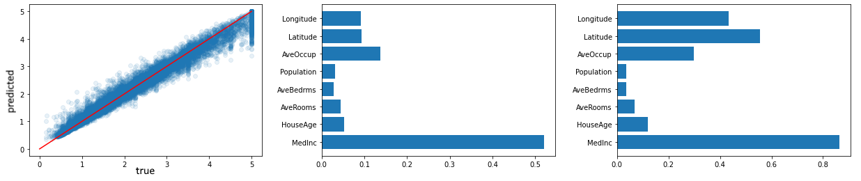
Note that this already highlights that permutation-based importance gives a less biased view.

Nevertheless, our focus is on discovery of interacting features. With the tools at our disposal, one would normally do so by:

• Inspecting univariate partial dependence plots for important features. Flatter (regions) in the plot might indicate that an interaction is going on
• Inspecting bivariate partial dependence plots
• Inspecting ICE plots

For example, taking a look at the ICE plot for HouseAge:

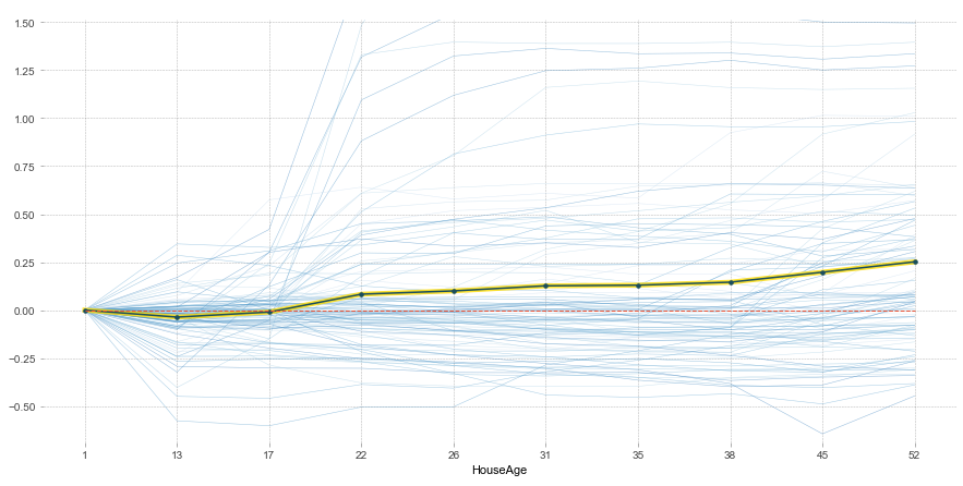
Shows that there is more going on than the univariate partial dependency would suggest. Bringing in another variable shows the following bivariate partial dependence plot:

plot_partial_dependence(model, X, [(
    list(X.columns).index('HouseAge'), 
    list(X.columns).index('AveRooms')
)])

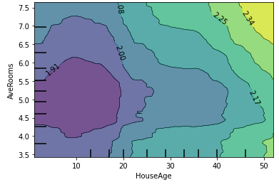
Indeed, on average the price increases for older houses, but we do see that it is strongly dependent on the AveRooms variable as well (e.g. for HouseAge between 30-40, the prediction ceteris paribus stays relatively flat, but not when taking into account the AveRooms feature).

For most uses cases, this is in fact quite sufficient to inspect models reasonably well. Still, let us now consider the H-measure ².

Using pdpbox

In the previous post, recall that we had modified pdpbox to calculate partial dependence values (our F values) for higher-order interactions. This still works with newer versions of pdpbox, and supports both using a given data set as well as a grid-based synthetic one, but sadly breaks down for non-toy data sets with more features as iterating over all possible feature set combinations becomes too computationally expensive.

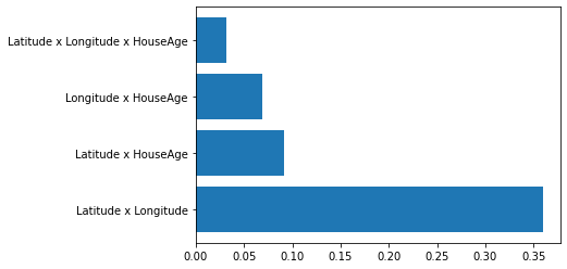
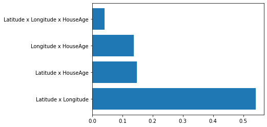
We can, however, limit ourselves to applying the second-order test on a chosen subset of features:

feats = ['Latitude', 'Longitude', 'HouseAge']

f_vals = compute_f_vals_pdpbox(model, X, feats=feats)

subsets = []
h_vals = []

for n in range(2, len(feats)+1):
    for subset in itertools.combinations(feats, n):
        h_val = compute_h_val(f_vals, subset)
        subsets.append(' x '.join(subset))
        h_vals.append(h_val)

plt.barh(range(len(h_vals)), h_vals, tick_label=subsets)

The reason for this is due to the fact that creating a synthetic data set over N features and m values per feature leads to m^N instances being created. Strangely enough, however, the implementation remains slow when using the given data set itself instead, as in:

f_vals = compute_f_vals(model, X, feats=X.columns, use_data_grid=True)

The reason for this is most likely due to pdpbox‘ internals (I suspect because of its tendency to calculate individual ICE-style dependencies and averaging those rather than a true PD approach).

Using scikit-learn

Since scikit-learn now supports partial dependence plots directly, we actually do no need to use pdpbox any longer. Note that plot_partial_dependence can only handle two-way interactions, but the partial_dependence function does in fact work with higher-order groups:

def center(arr): return arr - np.mean(arr)

def cartesian_product(*arrays):
    la = len(arrays)
    dtype = np.result_type(*arrays)
    arr = np.empty([len(a) for a in arrays] + [la], dtype=dtype)
    for i, a in enumerate(np.ix_(*arrays)):
        arr[...,i] = a
    return arr.reshape(-1, la)

def compute_f_vals_sklearn(model, X, feats=None, grid_resolution=100):

    def _pd_to_df(pde, feature_names):
        df = pd.DataFrame(cartesian_product(*pde[1]))
        rename = {i: feature_names[i] for i in range(len(feature_names))}
        df.rename(columns=rename, inplace=True)
        df['preds'] = pde[0].flatten()
        return df

    def _get_feat_idxs(feats):
        return [tuple(list(X.columns).index(f) for f in feats)]

    f_vals = {}
    if feats is None:
        feats = list(X.columns)

    # Calculate partial dependencies for full feature set
    pd_full = partial_dependence(
        model, X, _get_feat_idxs(feats), 
        grid_resolution=grid_resolution
    )

    # Establish the grid
    df_full = _pd_to_df(pd_full, feats)
    grid = df_full.drop('preds', axis=1)

    # Store
    f_vals[tuple(feats)] = center(df_full.preds.values)

    # Calculate partial dependencies for [1..SFL-1]
    for n in range(1, len(feats)):
        for subset in itertools.combinations(feats, n):
            pd_part = partial_dependence(
                model, X, _get_feat_idxs(subset),
                grid_resolution=grid_resolution
            )
            df_part = _pd_to_df(pd_part, subset)
            joined = pd.merge(grid, df_part, how='left')
            f_vals[tuple(subset)] = center(joined.preds.values)

    return f_vals

There are a couple of drawbacks here as well, the first one being that I’m taking a memory-hungry cartesian product of the results of partial_dependence, just so I can stick to the same synthetic grid and use pd.merge.

As such, we are limited to a second-order H-measure with a limited subset of features here as well. Trying to work around the cartesian product doesn’t even help a lot, as partial_dependence itself with run out of memory when trying to execute it on all features:

partial_dependence(model, X, [tuple(x for x in range(len(X.shape[1])))])

Note that you can lower the grid_resolution parameter (the default is a high 100), but in the end we’re still dealing with m^N instances being created. As a second drawback, the scikit-learn implementation does not support passing in your own custom grid.

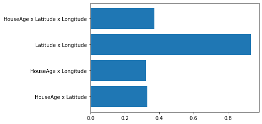
Still, we can apply it for a limited sets of features:

feats = ['Latitude', 'Longitude', 'HouseAge']

f_vals = compute_f_vals_sklearn(model, X, feats=feats)

subsets = []
h_vals = []

for n in range(2, len(feats)+1):
    for subset in itertools.combinations(feats, n):
        h_val = compute_h_val(f_vals, subset)
        subsets.append(' x '.join(subset))
        h_vals.append(h_val)

plt.barh(range(len(h_vals)), h_vals, tick_label=subsets)

The results are more or less comparable to the ones obtained using pdpbox (probably even a bit better as the default grid resolution of scikit-learn is higher by default).

Also, at least this approach is (barely) fast enough to brute force our way through all possible two and three-way interactions and rank them on their second-order H-measure (when using a lower grid resolution).

Manually

Finally, we can of course also calculate partial dependencies ourselves and stick to a given data set instead of creating synthetic examples.

def compute_f_vals_manual(model, X, feats=None):

    def _partial_dependence(model, X, feats):
        P = X.copy()
        for f in P.columns:
            if f in feats: continue
            P.loc[:,f] = np.mean(P[f])
        # Assumes a regressor here, use return model.predict_proba(P)[:,1] for binary classification
        return model.predict(P)

    f_vals = {}
    if feats is None:
        feats = list(X.columns)

    # Calculate partial dependencies for full feature set
    full_preds = _partial_dependence(model, X, feats)
    f_vals[tuple(feats)] = center(full_preds)

    # Calculate partial dependencies for [1..SFL-1]
    for n in range(1, len(feats)):
        for subset in itertools.combinations(feats, n):
            pd_part = _partial_dependence(model, X, subset)
            f_vals[tuple(subset)] = center(pd_part)

    return f_vals

It does make the results less precise, but this is fast and good enough for general exploration.

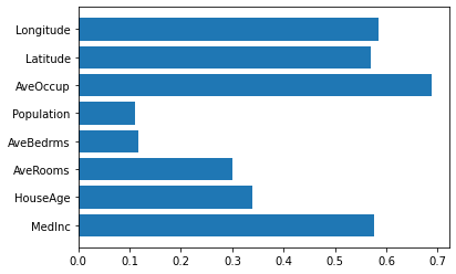
We can now perform our first order test:

subsets = []
h_vals = []

feats = list(X.columns)

f_vals = compute_f_vals_manual(model, X, feats=feats)

for subset in feats:
    h_val = compute_h_val_any(f_vals, feats, subset)
    subsets.append(subset)
    h_vals.append(h_val)

plt.barh(range(len(h_vals)), h_vals, tick_label=subsets)

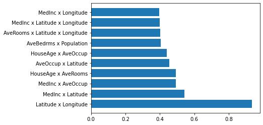
We can also show the top ten second order results:

subsets = []
h_vals = []

feats = list(X.columns)

for n in [2,3]:
    for subset in itertools.combinations(feats, n):
        h_val = compute_h_val(f_vals, subset)
        subsets.append(' x '.join(subset))
        h_vals.append(h_val)

subsets = np.array(subsets); h_vals = np.array(h_vals); k = 10
plt.barh(range(k), h_vals[h_vals.argsort()[::-1][:k]], tick_label=subsets[h_vals.argsort()[::-1][:k]])

Conclusion

As Christoph Molnar discusses in his interpretable ML book, the Friedman H-statistic is not perfect:

• It takes a long time to compute. Lower grid resolutions or sampling the data set can help
• It estimates marginal distributions, which have a certain variance and can vary from run to run
• It is unclear whether an interaction is significantly greater than 0, a model agnostic test is unavailable (an open research question)
• The interaction statistic works under the assumption that we can shuffle features independently. If the features correlate strongly, the assumption is violated and we integrate over feature combinations that are very unlikely in reality. This problem shows up for a lot of interpretability techniques, however
• The statistic is 0 if there is no interaction at all and 1 if all of the variance of the partial dependence of a combination of features is explained by the sum of the partial dependence functions. However, the H-statistic can also be larger than 1, which is more difficult to interpret