Fri 06 January 2017, by Seppe "Macuyiko" vanden Broucke
Our local Belgian media was just reporting on a study showing that air pollution has a negative impact on the cognitive abilities of children (link in Dutch).
With that in mind, I was reminded of the World Air Quality Index team, which keeps track of pollution values across the world. In Brussels, the index is (today) at 75. Well, if that’s bad, the index is >300 for Beijing.
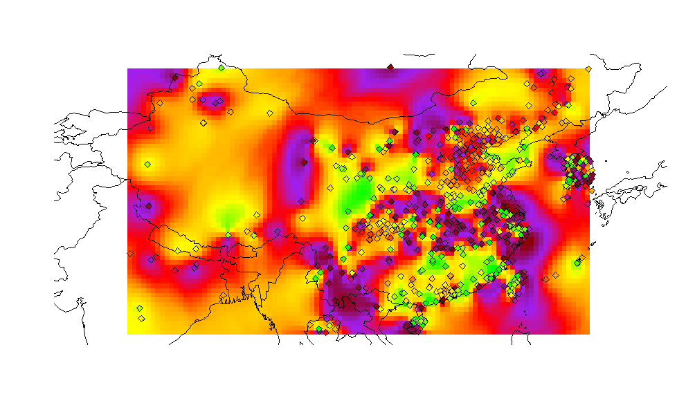
Seeing as I’ll be heading towards China again soon, I spend half an hour trying to have some quick fun with spatial kriging using this data set, also sometimes referred to as — or used to perform — spatial interpolation:
library(rworldmap)
library(rjson)
library(RCurl)
library(stringr)
library(kriging)

baseurl <- 'https://wind.waqi.info/mapq/bounds/?bounds={bounds}&inc=placeholders'
newmap <- getMap(resolution = "low")

bounds <- c(18.312810846425442,77.783203125,48.16608541901253,129.462890625)

jsondata <- getURL(str_replace(baseurl, '\\{bounds\\}', paste(bounds, collapse=',')))
jsondata <- do.call(rbind.data.frame, fromJSON(jsondata))
jsondata <- jsondata[jsondata$aqi != '-',]

model <- kriging(jsondata[,'lon'], jsondata[,'lat'], jsondata[,'aqi'])

plot(newmap, ylim = c(bounds[1], bounds[3]), xlim = c(bounds[2], bounds[4]), asp = 1)

colorRamp <- function(x, b=100) {
  rb <- colorRampPalette(c('green', 'yellow', 'orange', 'red', 'purple', 'darkred'))
  rb(b)[as.numeric(cut(x, breaks = b))]
}

model$map$col <- colorRamp(model$map$pred)
apply(model$map, 1, function(r) {
  points(r[['x']], r[['y']], pch=15, col=r[['col']])
})

plot(newmap, ylim = c(bounds[1], bounds[3]), xlim = c(bounds[2], bounds[4]), asp = 1, add = T)

jsondata$col <- colorRamp(as.numeric(jsondata$aqi))
apply(jsondata, 1, function(r) {
  points(r[['lon']], r[['lat']], pch=23, bg=r[['col']])
})