(This is part 2 in the Modern Genetic Algorithms Explained series, click here to go to the first post, or browse through all the parts with the Table Of Contents at the end of this post.)
Let’s take another look at the blog post on which we will base ourselves on. A general genetic algorithms can be described as follows:
Construct initial population
Repeat until time limit hit or satisfiable solution found:
  Assign a **fitness** score to each individual
  Use a **selection** method to pick individuals for reproduction
  Construct a new population, using a **crossover** method
  Use a **mutation** method to mutate the new population`
There are still a lot of gaps to fill in: how large should the population be, how do we construct individuals, which fitness function do we use, which selection methods are available, how do we evolve the population, should we mutate? If yes, and how?
Population and Individuals: Encoding and Construction
Let’s start with the population: if the population count is too low, there will not be enough diversity between the individuals to find an optimal or good solution. If the count is too high, the algorithm will execute slower, conversion to a solution might become slower as well. There is no ‘golden rule’ to find an optimal number.
How do we construct individuals? Certainly a simple (and popular choice) is the bit-representation:
0110 0111 0001 1011 ...
When evaluating the individuals, those bits are converted in something meaningful, be it numbers, strings, or other symbols, depending on the problem.
If we had used this representation, an individual for the problem described in the article (find x numbers each between a and b so that the summation of those numbers equal z) would look like this (e.g. x = 4):
01100111 01000101 11010101 11010111
Which would represent 4 numbers between zero and 255: 103+69+213+215. Also notice that our individuals have a fixed-length. Variable-length is a bit more complex, but also possible, and sometimes needed.
What do we do if the number lies out of the permitted bounds? We could: (1) Avoid that situation by making sure we never generate an individual with a number < a or > b. (2) Permit those individuals, but assign a very low fitness score to them. In the article, the score is calculated as the absolute difference between the sum of the individual’s numbers and the target value. So a score zero (0) means perfect fitness: a valid solution. In this case, invalid individuals would get a score of 1000, for example. Or even better, we evaluate it normally, but then add a “penalty”. E.g. the absolute difference between the bounds and the numbers times two.
Why would we use (2)? In some cases it is too difficult or too time-consuming to check every individual to see if it is valid, before putting it in the population pool. Also: permitting invalid individuals might still be useful. They can introduce more variety in the population, and their valid parts can still be used to create offspring.
Why would we use this representation? As we will see in the following steps, a crossover between two individuals will happen to create new offspring, with a bit representation, the crossover point can be placed at any point:
             v
01100111 010 | 00101 11010101 11010111
01101111 000 | 00100 10010111 10011100
When we use a list of integers, we place the crossover point between two numbers, this is different from the previous example, where the crossover point could be arbitrarily placed “in the middle of a number”:
    v
103 | 69 , 213 , 215
13  | 22 , 123 , 76
Bit-representation is thus often used when it is not clear how to place the crossover point, but when we do know a way to “convert” a solution to a bitstring. However, always watch out. Some representations become too sensitive to “random” tinkering with bits, making them quickly invalid. In our case: using a bit-representation would be permitted (changing a random bit still creates four integers), but in other cases this method becomes unfeasible.
Selection
Good, we now have constructed an initial population, containing, say 100, individuals. We also have a fitness function to assign a score to each of them. Lower is better, 0 being a perfect solution.
How do we pick individuals to use to create offspring? We’ll need two individuals (a father and a mother). A first way (1) to choose them might be: just pick them at random. Of course, it is ease to see that this is a bad way of choosing parents. There has to be a relation between the fitness and the selection, so that better offspring can be created. When we choose parents at random, bad parents have an equal chance of producing children than fitter parents. (This is against the ‘survival of the fittest’-idea, on which genetic algorithms are based on.)
In the article, a second (2) method is used:
Pick the n-best individuals from our current population
Pick two different random individuals from those n-best
Use those as parents for a child
This is certainly a better option, but this way, we completely abandon the lower scoring individuals. It is always better to give even the worst individuals a little chance to be a parent, to maintain a higher level of possible diversity.
With that remark in mind, we arrive at a third (3) solution, the roulette-wheel selection method: the chance of each individual to be selected becomes: fitness of that individual / total of fitness scores of every individual in the population. For example, consider the following population of five individuals, ordered by their score (let’s say that higher is better).
i3: 9
i2: 7
i5: 6
i4: 3
i1: 1
Total: 26
Now pick a random value between zero and 26. Let’s say 8: 8 > 1, continue; 8 > 1 + 3, continue; 8 > 1 + 3 + 6, we pick i5. It’s easy to see where the name “roulette selection” comes from.
Another selection method (4) is called tournament selection:
Choose k (the tournament size) individuals from the population at random
  Choose the best individual from pool/tournament with probability p
  Choose the second best individual with probability p*(1-p)
  Choose the third best individual with probability p*((1-p)^2)
  ...
Note that p can be = 1. Then the best out of k individuals is chosen, this is fairly common. For k, often 2, 3, or 4 is used. This is an often-used method because it is easy to implement, and can be used in parallel environments. Note that when p = 1, k = 1 this method essentially becomes a pure random selection.
Crossover
Now that we know how to select two parents, how do we create children? Again, there are many techniques here. The first one (1) is the one-point crossover (simple crossover). I will illustrate the following examples with bit-represented individuals.
                    v
0000 0000 0000 0000 | 0000 0000
1111 1111 1111 1111 | 1111 1111
Creates two children:
                    v
0000 0000 0000 0000 | 1111 1111
1111 1111 1111 1111 | 0000 0000
The crossover point can be randomly chosen, or can be a fixed location (1/4, 1/3, 1/2 are commonly used). After the crossover point, two children are created by swapping their bits.
The second (2) crossover method is two-point crossover, and looks a lot like the previous method:
     v                v
0000 | 0000 0000 0000 | 0000 0000
1111 | 1111 1111 1111 | 1111 1111
Creates two children:
     v                v
0000 | 1111 1111 1111 | 0000 0000
1111 | 0000 0000 0000 | 1111 1111
Again: it’s swap - and swap.
Cut and splice (3) is another one, and is only interesting when you need variable-length individuals. I will skip the description, it’s in the Wikipedia page (all sources are mentioned at the end of this post).
UX (Uniform Crossover) (4) is a bit more interesting:
1111 1111 1111 0000 0000 0000
1111 1111 1111 1111 1111 1111
Creates two children:
1111 1111 1111 0010 1101 0100
1111 1111 1111 1101 0010 1011
It works as such: every bit has a 0.5% chance of swapping. Of course, if both parents have a bit 0 or 1, it stays 0 or 1.
HUX (Half Uniform Crossover) (5) swaps exactly half of the non-matching bits. So pick N/2 bits out of N non-matching bits, and swap them.
In our reference article, a single fixed crossover point is used, placed in the middle.
Mutation
Now that that’s out of the way, there is only one aspect to look at: mutation. This phase makes sure that there is enough randomness and diversity in the population. Again, there are different options.
First (1) of all: no mutation. For example when their is enough diversity by using smart selection and crossover methods, or when the optimization problem is as such that there are no local maxima (more about that a bit later).
A second (2) method: take N individuals out of our population, and change each of their bits/values with a P chance. Often: N is equal to the complete population size, with P a very small value. Or:
(3) Take N individuals, pick K bits/values in every individual, and change those bits/values. Again: N is often equal to the complete population, and K also low (one for example). This is the method used in the article.
Sometimes, also the following additional (4) method is used: create offspring equal to (P-N), with P being to population size and 0<=N<=P, then add N random individuals. When this method is used, often values like N=P/5 to P/10 are used.
In Action
That’s it, we’re done! Let’s see a few action examples of genetic algorithms.
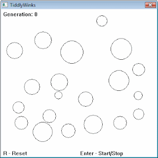
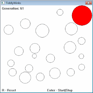
A problem involves: given a constrained plane and a few randomly placed circles, how can we place another circle so that the radius is maximal, without overlapping the other circles. You can download and try it for yourself here (all sites are also mentioned at the end of this post).
Before the evolution starts, the situation looks like this:
After only 61 generations, we are coming close to the optimum:
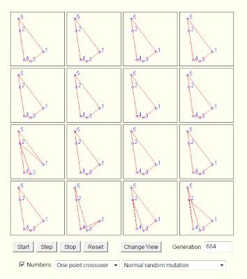
Another really cool example can be found here. Be sure to download the binary and test it for yourself:

This site implements a Traveling Salesman Solver with a GA Java applet:
Finally, using the code from the article:
import sys
  sys.path.append("C:\Users\Seppe\Desktop")
  from genetic import *
  target = 300
  p_count = 100
  i_length = 5
  i_min = 0
  i_max = 100
  p = population(p_count, i_length, i_min, i_max)
  fitness_history = [grade(p, target),]
  for i in xrange(100):
    p = evolve(p, target)
    fitness_history.append(grade(p, target))

  for datum in fitness_history:
    print datum
Outputs:
66.51
28.84
19.41
18.66
11.97
13.26
5.41
1.15
1.5
1.55
2.9
3.0
0.3
0.0
0.0
0.0
...
After 14 evolutions we already see a perfect population, not bad… Do note however that this is an extremely easy problem: there are many optimum solutions.
Remarks and Problems
Genetic Algorithms are not perfect, nor are they a silver bullet. When badly configured, genetic algorithms tend to expose the same flaws as stochastic hill climbing indeed: a tendency to converge towards local optima.
Consider the following function:
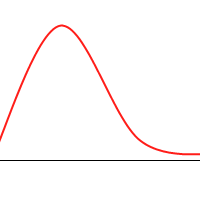
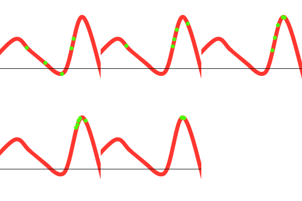
It’s not hard to construct a GA which will tend toward the global maximum, even without mutation or introducing much diversity. Consider the following animation, with the green dots representing a few individuals:

However, when you consider the following function:

We might get lucky and end up with:
Notice that there is one individual tending towards the local maximum, but the others “pull” it towards the global one. However, the following could also happen:
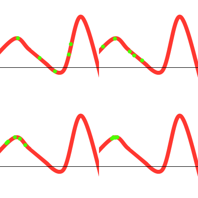
To prevent these situations from happening, we have various options at our disposal: (1) Choose sensible parameters. Population count, selection- crossover- and mutation-methods. Try to find a balance between enough diversity and fast convergence. (2) Run the GA multiple times, take the best solution. (3) If the population converges towards a certain solution, randomly regenerate the N worst members of the population and continue evolution (a similar technique could be used in the mutation stage). (4) Use parallel solutions. A parallel genetic algorithm executes multiple populations at once, often on many computers (or a cluster). Often, there is an extra migration stage added, in which individuals migrate from one population to another.
Sources
Wow, what a lot of text! If you’re interested in knowing more, check the following links:
- The original article which inspired this text.
- Wikipedia also has lots of information: Genetic algorithms, Selection (Roulette and Tournament), Crossover and Mutation.
- An old tutorial on ai-junkie (but still useful). Back in the day, this was the first thing I read about genetic algorithms.
- Another old website, made by Marek Obitko, still, the information contained is relevant and interesting. Also hosts the TSP Java applet.
- This opendir contains university slides about emerging computing technologies. A032 talks about genetic algorithms. The slides are ugly as hell, but contain some good information! (There is a part about CHC Eshelman, which we will discuss in the next part in this series).
- This Powerpoint file contains some information about CHC Eshelman as well. The file is not that interesting, but does contain a good example on crossover feasibility: sometimes our individuals are encoded as such that they can become invalid after each crossover. We must then “normalize” or correct parents or children to produce valid offspring. We mentioned this problem in the above post.
- Evolution of Mona Lisa, check this!
There are a lot of software implementations around for genetic algorithms, most of them are written in C, C++ or FORTRAN77, but recently languages such as Java and Python are becoming more popular.
Check Wikipedia’s External links for more tutorials and software libraries.
In the next section: we will explore a particular GA implementation: CHC by Eshelman.
Table Of Contents (click a link to jump to that post)
1- Introduction 2- Genetic Algorithms 3- CHC Eshelman 4- Simulated Annealing 5- Ant Colony Optimization 6- Tabu Search 7- Conclusion