Update: this post now has a follow-up with some further details.

Throughout the past year or so, both R and Python focused data science practioners have picked up on a paper by Friedman and Popescu from 2008 entitled Predictive Learning Via Rule Ensembles. Interestingly enough, the “meat” of the paper — at least in the context we’ll discuss here — is found in the latter half, where a helpful statistic is proposed to assess interaction effects between variables in an ensemble model ¹.

Together with feature importance rankings and partial dependence plots, getting an idea of which variables interact is an effective means to make black-box models more understandable, especially since the latter can effect how you look at the former two.

The reason why I initially became interested in this idea was in a setting where a well-performing random forest model had to be converted to a (hopefully just as well performing) logistic regression model for deployment reasons. In this setting, getting some insights from the ensemble model in terms of which variables (and associated interaction effects) to keep is quite useful.

Feature Importance

Let us begin with outlining some basic concepts first, assuming some knowledge regarding predictive (ensemble) models.

First, there’s the idea of feature importance ranking, as mentioned above. We don’t necessarily need it to discuss the remainder of this post, though it’s still a good idea to discuss it as we’ll see later where it can fall short.

Say you have trained a complex ensemble model (e.g. a random forest containing a couple hundred decision trees) and you want to get an idea of which features were “important” in the model. In a univariate setting, one might simply take a look at a χ2 test or correlations, though given how a base learner like a decision tree is good to pick up on non-linearities, most practitioners prefer to “let the model do the talking” instead.

A common method to do so is to use a particular implementation of “feature importance” based on “permutations” (as this works with any model, compared to other approaches which assume that the ensemble is a bag).

The idea works as follows. Say you’ve just trained a model using a feature matrix X, row/column indexed as X[i,j]. To assess the importance of a variable j, we can compare a metric of interest (accuracy or AUC, or anything else really) on X with a modified instance it ², X’, where we permute, i.e. shuffle, the column j.

This idea was already described by Breiman and Cutler in their original random forest paper as an alternative for Gini-decrease based feature importance. In other words, the idea is to permute the column values of a single feature and then pass all samples back through the model and recompute the accuracy (or AUC, or R2, or…) The importance of that feature is the difference between the baseline and the drop in overall accuracy caused by permuting the column. The more important that feature was for the model, the higher the drop in accuracy will be.

This is a very simple mechanism, though computationally expensive, but very much — again — the preferred approach in practice. In fact, alternative implementations have been proven to be quite biased in many implementations, as well as harder to set up (as it might involve retraining the model several times). Also see this fantastic post from 2018 which delves into the topic of feature importance in depth. I fully recommended going to the post, in fact, if you’ve been using feature importance in your working, as many implementations (both in R and Python) will default to using the biased technique. Let me even go ahead and quote:

The scikit-learn Random Forest feature importance and R’s default Random Forest feature importance strategies are biased. To get reliable results in Python, use permutation importance, provided here and in our rfpimp package (via pip). For R, use importance=T in the Random Forest constructor then type=1 in R’s importance() function. In addition, your feature importance measures will only be reliable if your model is trained with suitable hyper-parameters.

In Python, you can also use the eli5 package to get solid feature importance rankings. An implementation in scikit-learn is also available, though not really in an “out of the box” fashion. (Also see this issue on GitHub.) (Update: scikit-learn has now finally implemented this as well as partial dependence plots.)

To get back on track, the permutation based feature importance ranking is solid (at least when used correctly) and easy to understand, with the drawback that it is quite computationally expensive. A theme which will remain for other things we’ll visit in this post as well, though which is a fair constraints whilst in the “model inspection” phase of your model development pipeline. (Jeremy Howard has also spoken quite a bit about this topic in the latest fast.ai courses on structured machine learning, and also indicates that sampling is fine; you’re doing inspection after all.)

As a final note, one might consider using an out-of-bag (OOB) or a validation set to assess feature importance rankings, though I’ve commonly encountered usage of the training set as well (again, we’re not necessarily trying to assess generalization performance, we just want to get an insight on our model, based on how — and on which data — it was trained). Even this fantastic book on model interpretabily argues that both train and test data might be valid depending on the use case.

The Trouble with Single-variable Importance Rankings

Feature importance rankings are great, but they’re not all-revealing. A common practice for instance is to use random forests or other ensemble models as a feature selection tool by first training them on the full feature set, and then using the feature importance rankings to select the top-n variables to keep in the productionized model (and hence retraining the model on the selected model). Think data-driven feature selection. This is a somewhat common approach which has been operationalized in packages such as Boruta.

The problem, however, is that it is easy to drop features using this strategy in case when they interact with other features.

As an example, let us construct a synthetic data set where y ~ x0 * x1 + x2 + noise. I.e. x0 and x1 interact. If we train a random forest or gradient boosting model even such a simple data set and assess the feature importance scores using scikit-learn, the problem becomes clear:

print(gbr.feature_importances_)
print(rfr.feature_importances_)

gradient boosting rankings:     [0.17174317, 0.19054922, 0.6377076 ]
random forest rankings:         [0.19065131, 0.18586131, 0.62348737]

scikit-learn doesn’t implement permutation based importance rankings (at the time of writing; note that feature_importances_ uses impurity based importance), but using rfpimp yields a similar result:

gradient boosting rankings:     [0.35668364, 0.37945421], 1.17092419]
random forest rankings:         [0.42673270, 0.43211179], 1.24873006]

Again, as we’ve stated, one needs to be careful using feature importance implementations as-is: variable x2 gets all the attention whilst the importance of the first two variables seems rather weak.

Nevertheless, by just looking at our data and plotting x0 and x1 versus the target (colored), we do see a strong interaction effect:

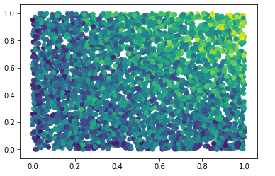
The question is now how we can uncover such effects by stepping beyond feature importance.

One idea we could explore is to modify the feature importance mechanism by permuting more than one variable at once. This is an interesting idea not widely explored in practice (it’s funny how even practioners never step outside of the even rudimentary bounds implementations are offering), though might nevertheless become wieldy for data sets with a considerable amount of features, especially when three-way or higher-order interaction effects need to be considered.

(As an aside, for ensemble models using decision trees as their base learner, i.e. the majority, other interesting investigations such as looking at the number of times a feature appears over the trees and how high it appears in the trees can provide valuable insights as well. Airbnb already played around with such ideas in 2015. It speaks highly to their engineering team that they were working on such things before “interpretable machine learning” was rediscovered by the rest of the community.)

There is an alternative offered by Friedman and Popescu, however, which can be implemented in a more systematic manner, and what we will focus on hereafter. First, we need to introduce an additional concept.

Partial Dependence Plots

Knowing which features play an important role is helpful (disregarding the interaction aspect for a bit longer). The next question one will be asked is commonly “why” or “how” these are important. An easy mistake to make is to think linearly and to think that if x goes up, y will go up (or down), though this ignores all those non-linear effects these black-box models are so good at extracting.

Instead, it makes more sense to draw up a partial dependence plot. The basic idea is simple as well. Given a variable j you are interested in (e.g. one established as being important, though any variable can be considered), we construct a synthetic data set as follows:

• For all variables k =/= j, we take their average (or median) value (or mode, for categoricals)
• Next, we “slide” over the variable j between its min and max values observed in the data, hence generating a new set of instances which only differ in their j feature
  • Note that this can either be grid based (e.g. a stepwise slide), or based on the actual values observed in the data
• We then ask the model to predict a probability for each row in our synthetic data set and plot the results (i.e. across the different values for j)

The idea is to get a ceteris paribus effects plot for this variable.

Trying this on our synthetic data set, we get:

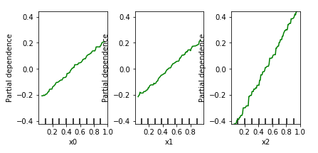
This idea works well in practice, though basically suffers from the same drawback as feature importance: we’re looking at the ceteris paribus effect per variable, in a univariate manner. Indeed, looking at the partial dependence plots above, one might get the impression that the effects of x0 and x1 are “less strong” than x2. This is a dangerous mistake to make. In general, one should understand that if you see a relationship, this indeed indicates presence of an effect on the target, though absence of a relationship does not indicate absence of an effect. In the extreme case, one might even observe a flat line for one of the variables involved in an interaction in the partial dependence plots, even though those variables together do impose a strong effect on the target.

Again, people have been aware of this drawback for quite a while. Forest floor was one of the first to pick up on this in the R world (since 2015 and a paper in 2016), and produced a package to plot two-way interaction effects. The pdp R package does something similar. Another package, for Python, sklearn_gbmi also allows to plot two-dimensional partial dependence plots, and so does pdpbox for Python. (Update: and recent versions of scikit-learn allow to plot two-dimensional partial dependence plots as well.)

The idea remains the same: keep everything ceteris paribus except for — now — two variables which we assess over a grid, either stepwise generated or based on the real values observed in the data.

Nevertheless, this is somewhat limited to two dimensions only; for three-way interaction effects and higher, one needs to get quite creative with colors and shapes to visually inspect the results.

ICE (Individual Conditional Expectation) Plots

ICE plots are a newer though very similar idea to partial dependence plots, but offer a bit more in terms of avoiding the “interaction” trap.

The idea here is not to “average” over variables k =/= j outside the variable of interest, but instead to keep every instance as is and slide over variable j of interest. Every original observation in the data set is hence duplicated with the variable j taking on multiple values, again either over a grid or based on the values observed in the data. The idea is then to plot a separate line for each original observation as we slide through the values of j on the x-axis.

This allows us to easily spot deviations across different segments of our population. For instance, this is the ICE plot for sliding over x0 in our synthetic data set:

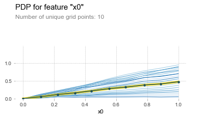
This is a very powerful concept, as it allows us to get the best results so far in a univariate setting. First, in case there are interaction effects (or general instabilities in predictive results) present, we can observe this in the ICE lines being “spread out” over the different values of j.

(Note: it is common practice to “center” the ICE lines at zero to make this comparison easier, as seen in the picture.)

Second, we can still easily extract a general “partial dependence style” plot by averaging the value across the lines, as displayed by the center yellow line in the picture above.

(Not that there would necessarily be any guarantee for this average ICE line to be exactly the same as the partial dependence plot as described above. It depends somewhat on the intricacies of the learner, though averages are such a… well, central, concept in virtually all learners that the results will be virtually similar. Again, this would make for a nice topic to explore further both from an empirical and theoretical perspective.)

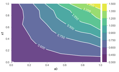
In any case, we now have the building blocks required to finally delve into what we’re interested in here. As one can observe, ICE plots are better suited to warn a user against interpreting a “partial dependency”, though can still make it quite hard to uncover the full extent of interactions. Again, when limiting oneself to the setting of two features, the concept of ICE plots is easily ported. This is the result for x0 * x1, for instance. The ICE plot clearly indicates the presence of an interaction, as would a standard partial dependence plot:

Though again, the question remains: how do we systematically extract deeper interactions, given that visualizations cannot help us much in this setting ³?

Introducing Friedman’s H-statistic

The interpretable ML book by Christoph Molnar actually gives us a workable approach, by using Friedman’s H-statistic based on decomposition of the partial dependence values.

The book describes both “versions” of the H-statistic:

• H2(jk) to measure whether features j and k interact. For this, partial dependence results need to be calculated for j and k separately, and j and k together. I’ll call this the second-order measure
• H2(j) to measure if a feature j interacts with any other feature. This can hence be regarded as a first-order measure guiding the second-order measures to check

This is a great approach, but two problems exist in most implementations:

• The second-order H2 measure can actually be constructed for higher-order interactions as well, the paper mentions this in passing through “Analogous relationships can be derived for the absence of higher order interactions” and by providing a metric for H2(jkl). This requires partial dependence values for higher-order feature sets, which most implementations do not provide
• Most implementations will only implement H2(jk), without providing the first-order test H2(j), which would greatly help to reduce the number of checks to perform

There are other aspects to consider as well (e.g. with regards to sampling to speed up the procedure), but let us focus on these for now and see which options are available.

• In R, the iml package implements both measures, but does not allow to calculate the second-order H-measure on higher-order feature sets, e.g. H2(jkl)
• The R interact.gbm package only works for gradient boosting models and does not implement the first-order measure, but does allow for higher-order second-order measures
• The R pre package seems to implement the first-order measure, but not the second-order one
• In Python, sklearn_gbmi will accept feature sets of length two and higher, but does not provide support for the first-order measure, very similar to interact.gbm in R. It only works on gradient boosting based models
• In Python, the vip implements a clever alternative approach to find whether two feature interact based on ICE plot comparisons which is much faster, but is only implemented for two-way interactions as well

A manual Python implementation

Especially in Python, the situation regarding the H-measure looks a bit bleak. Using pdpbox to extract partial dependence values, we can however set up an implementation of both measures which work for any model. For two-way interactions (hiding the exact calculation of the H-measure until a bit later), we can compare our result with what sklearn_gbmi tells us for H2(jk):

gradient boosting (first result is sklearn_gbmi, second is ours):
('x0', 'x1') 0.3694527407798142     0.21799393342197507
('x0', 'x2') 0.04741546008708799    0.037965435191138985
('x1', 'x2') 0.0350484030284537     0.03754977728770199

random forest:
('x0', 'x1')                        0.252313467519671
('x0', 'x2')                        0.03840902079127481
('x1', 'x2')                        0.034315016474317464

Small differences are due to handling of the construction of the values for the features under observation to “slide” over. sklearn_gbmi uses the values as seen in the data set whereas pdpbox using a grid based approach, but the results are comparable: both models show that variables x0 and x1 interact.

However, for H2(jkl) and higher-order interactions, we need to modify pdpbox so that is is able to calculate partial dependence values for more than two variables under consideration. (In fact, pdpbox does silently accept more than two features when calling it, but will simply ignore everything apart from the first two.)

As such, we define a function as follows:

from pdpbox.pdp_calc_utils import _calc_ice_lines_inter
from pdpbox.pdp import pdp_isolate, PDPInteract
from pdpbox.utils import (_check_model, _check_dataset, _check_percentile_range, _check_feature,
                    _check_grid_type, _check_memory_limit, _make_list,
                    _calc_memory_usage, _get_grids, _get_grid_combos, _check_classes)
from joblib import Parallel, delayed

def pdp_multi_interact(model, dataset, model_features, features, 
                    num_grid_points=None, grid_types=None, percentile_ranges=None, grid_ranges=None, cust_grid_points=None, 
                    cust_grid_combos=None, use_custom_grid_combos=False,
                    memory_limit=0.5, n_jobs=1, predict_kwds=None, data_transformer=None):

    def _expand_default(x, default, length):
        if x is None:
            return [default] * length
        return x

    def _get_grid_combos(feature_grids, feature_types):
        grids = [list(feature_grid) for feature_grid in feature_grids]
        for i in range(len(feature_types)):
            if feature_types[i] == 'onehot':
                grids[i] = np.eye(len(grids[i])).astype(int).tolist()
        return np.stack(np.meshgrid(*grids), -1).reshape(-1, len(grids))

    if predict_kwds is None:
        predict_kwds = dict()

    nr_feats = len(features)

    # check function inputs
    n_classes, predict = _check_model(model=model)
    _check_dataset(df=dataset)
    _dataset = dataset.copy()

    # prepare the grid
    pdp_isolate_outs = []
    if use_custom_grid_combos:
        grid_combos = cust_grid_combos
        feature_grids = []
        feature_types = []
    else:
        num_grid_points = _expand_default(x=num_grid_points, default=10, length=nr_feats)
        grid_types = _expand_default(x=grid_types, default='percentile', length=nr_feats)
        for i in range(nr_feats):
            _check_grid_type(grid_type=grid_types[i])

        percentile_ranges = _expand_default(x=percentile_ranges, default=None, length=nr_feats)
        for i in range(nr_feats):
            _check_percentile_range(percentile_range=percentile_ranges[i])

        grid_ranges = _expand_default(x=grid_ranges, default=None, length=nr_feats)
        cust_grid_points = _expand_default(x=cust_grid_points, default=None, length=nr_feats)

        _check_memory_limit(memory_limit=memory_limit)

        pdp_isolate_outs = []
        for idx in range(nr_feats):
            pdp_isolate_out = pdp_isolate(
                model=model, dataset=_dataset, model_features=model_features, feature=features[idx],
                num_grid_points=num_grid_points[idx], grid_type=grid_types[idx], percentile_range=percentile_ranges[idx],
                grid_range=grid_ranges[idx], cust_grid_points=cust_grid_points[idx], memory_limit=memory_limit,
                n_jobs=n_jobs, predict_kwds=predict_kwds, data_transformer=data_transformer)
            pdp_isolate_outs.append(pdp_isolate_out)

        if n_classes > 2:
            feature_grids = [pdp_isolate_outs[i][0].feature_grids for i in range(nr_feats)]
            feature_types = [pdp_isolate_outs[i][0].feature_type  for i in range(nr_feats)]
        else:
            feature_grids = [pdp_isolate_outs[i].feature_grids for i in range(nr_feats)]
            feature_types = [pdp_isolate_outs[i].feature_type  for i in range(nr_feats)]

        grid_combos = _get_grid_combos(feature_grids, feature_types)

    feature_list = []
    for i in range(nr_feats):
        feature_list.extend(_make_list(features[i]))

    # Parallel calculate ICE lines
    true_n_jobs = _calc_memory_usage(
        df=_dataset, total_units=len(grid_combos), n_jobs=n_jobs, memory_limit=memory_limit)

    grid_results = Parallel(n_jobs=true_n_jobs)(delayed(_calc_ice_lines_inter)(
        grid_combo, data=_dataset, model=model, model_features=model_features, n_classes=n_classes,
        feature_list=feature_list, predict_kwds=predict_kwds, data_transformer=data_transformer)
                                                for grid_combo in grid_combos)

    ice_lines = pd.concat(grid_results, axis=0).reset_index(drop=True)
    pdp = ice_lines.groupby(feature_list, as_index=False).mean()

    # combine the final results
    pdp_interact_params = {'n_classes': n_classes, 
                        'features': features, 
                        'feature_types': feature_types,
                        'feature_grids': feature_grids}
    if n_classes > 2:
        pdp_interact_out = []
        for n_class in range(n_classes):
            _pdp = pdp[feature_list + ['class_%d_preds' % n_class]].rename(
                columns={'class_%d_preds' % n_class: 'preds'})
            pdp_interact_out.append(
                PDPInteract(which_class=n_class,
                            pdp_isolate_outs=[pdp_isolate_outs[i][n_class] for i in range(nr_feats)],
                            pdp=_pdp, **pdp_interact_params))
    else:
        pdp_interact_out = PDPInteract(
            which_class=None, pdp_isolate_outs=pdp_isolate_outs, pdp=pdp, **pdp_interact_params)

    return pdp_interact_out

And can now call:

pdp_multi_interact(gbr, tr_X, xs.columns, ['x0', 'x1', 'x2'])

    x0          x1          x2          preds
0   0.000356    0.000016    0.000074    -0.122989
1   0.000356    0.000016    0.111043    -0.005618
2   0.000356    0.000016    0.220973    0.149123
3   0.000356    0.000016    0.338448    0.305684
...

Next, we implement a function to calculate F values (i.e. partial dependence values) for (jkl…) and all subsets:

def center(arr): return arr - np.mean(arr)

def compute_f_vals(mdl, X, features, selectedfeatures, num_grid_points=10, use_data_grid=False):
    f_vals = {}
    data_grid = None
    if use_data_grid:
        data_grid = X[selectedfeatures].values
    # Calculate partial dependencies for full feature set
    p_full = pdp_multi_interact(mdl, X, features, selectedfeatures, 
                                num_grid_points=[num_grid_points] * len(selectedfeatures),
                                cust_grid_combos=data_grid,
                                use_custom_grid_combos=use_data_grid)
    f_vals[tuple(selectedfeatures)] = center(p_full.pdp.preds.values)
    grid = p_full.pdp.drop('preds', axis=1)
    # Calculate partial dependencies for [1..SFL-1]
    for n in range(1, len(selectedfeatures)):
        for subsetfeatures in itertools.combinations(selectedfeatures, n):
            if use_data_grid:
                data_grid = X[list(subsetfeatures)].values
            p_partial = pdp_multi_interact(mdl, X, features, subsetfeatures, 
                                        num_grid_points=[num_grid_points] * len(selectedfeatures),
                                        cust_grid_combos=data_grid,
                                        use_custom_grid_combos=use_data_grid)
            p_joined = pd.merge(grid, p_partial.pdp, how='left')
            f_vals[tuple(subsetfeatures)] = center(p_joined.preds.values)
    return f_vals

From which we can define the second-order H-measure:

def compute_h_val(f_vals, selectedfeatures):
    denom_els = f_vals[tuple(selectedfeatures)].copy()
    numer_els = f_vals[tuple(selectedfeatures)].copy()
    sign = -1.0
    for n in range(len(selectedfeatures)-1, 0, -1):
        for subfeatures in itertools.combinations(selectedfeatures, n):
            numer_els += sign * f_vals[tuple(subfeatures)]
        sign *= -1.0
    numer = np.sum(numer_els**2)
    denom = np.sum(denom_els**2)
    return math.sqrt(numer/denom) if numer < denom else np.nan

And first-order H-measure as well:

def compute_h_val_any(f_vals, allfeatures, selectedfeature):
    otherfeatures = list(allfeatures)
    otherfeatures.remove(selectedfeature)
    denom_els = f_vals[tuple(allfeatures)].copy()
    numer_els = denom_els.copy()
    numer_els -= f_vals[(selectedfeature,)]
    numer_els -= f_vals[tuple(otherfeatures)]
    numer = np.sum(numer_els**2)
    denom = np.sum(denom_els**2)
    return math.sqrt(numer/denom) if numer < denom else np.nan

Testing this on one of our models, we get, for the first-order H measure:

x0 is in interaction: 0.2688984990347688
x1 is in interaction: 0.26778914050926556
x2 is in interaction: 0.10167180905369481

We can then calculate the second-order H-measure, also for higher-order interactions:

gradient boosting (first result is sklearn_gbmi, second is ours):
('x0', 'x1')        0.3694527407798142      0.3965718336359157
('x0', 'x2')        0.04741546008708799     0.04546491988445405
('x0', 'x1', 'x2')  0.030489287134804244    0.028760391025931864

random forest:
('x0', 'x1')                                0.42558760788710415
('x0', 'x2')                                0.05978441740731955
('x0', 'x1', 'x2')                          0.07713738471773776

And that’s it; a lot of “set-up” for a relatively simple payoff, though it does reveal how a deep understanding of the techniques you use is necessary to know in which cases they can fail, as well as the importance of taking a look at implementations to see what exactly they implement and what they do not.

In my search on “white washing” black box models, I also discovered the following clever approaches:

• RuleFit: a technique which combines linear models with new features learnt using decision trees that represent interactions
• skope-rules: a trade off between the interpretability of a Decision Tree and the power of a Random Forest, which offers a very interesting approach as well aimed at deriving a short list of precise rules