I’ve been spending way too much time with Oxygen Not Included. It’s a great and addictive base building game with lots of challenges to tackle, though the most interesting component — for me, at least — is the way how the game simulates the behavior of gasses, liquids, temperature, and elektricity.

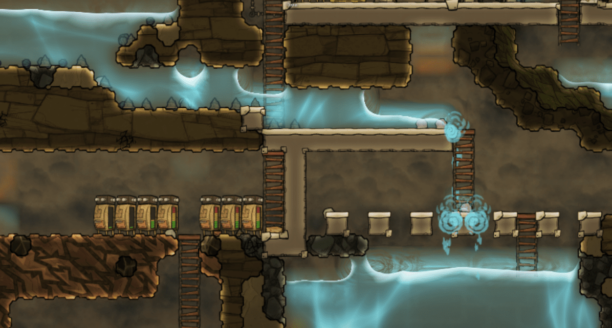
Oxygen Not Included is certainly not the only game incorporating similar systems. Minecraft, of course, does the same with water, lava, and redstone (albeit in different ways), and so do other games like Cities: Skylines and the more recent SimCity incarnation:

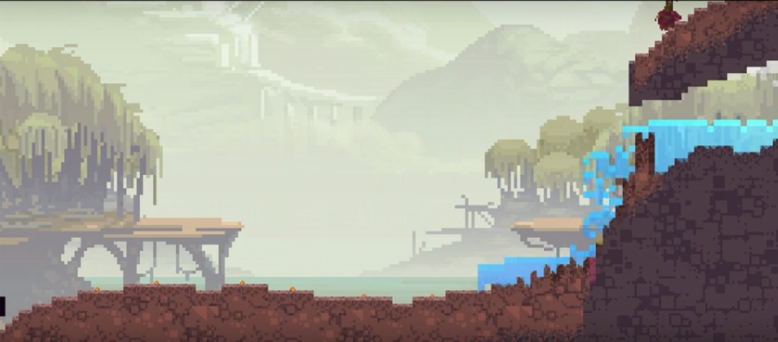
Once you start noticing these systems, you see them popping up everywhere, from simple mobile games like The Sandbox to little “falling sand” web games.

Many of these games’ systems are based on the same underlying fundamentals. In this series of articles, I’ll go through explaining two popular concepts and how they work inside such games: cellular automata, and graphs. As a side goal, I also wanted to take the opportunity to play around a bit with p5.js to visualize and create such systems.

Cellular automata

Cellular automata have been around for quite some time already (originally discovered in the 1940s by Stanislaw Ulam and John von Neumann). A cellular automaton is a “discrete model, consisting of a regular grid of cells, each in one of a finite number of states” (Wikipedia). For each cell, a set of cells called its neighborhood is defined relative to the specified cell. From an initial state, a simulation is started where each new generation is created according to a set of rules that determines the new state of each cell in terms of the current state of the cell and the states of the cells in its neighborhood. In basic terms, this defines a “main loop” over our grid as follows:

forever:
    for each current cell in current grid:
        get current neighborhood
        determine state for new cell based on current cell and current neighborhood
    swap new grid to current grid

That’s the basic idea, and it’s this system that is driving all the water, sand, … systems in the games listed above. Of course, the main interestingsness from using this approach comes from the pieces left to you to plug in, namely:

• How you define the neighborhood of a cell
• How you define the state of a cell
• How you define the rules to determine the state in a new generation

Let’s start by implementing this basic idea in JavaScript using p5.js. First, let’s define a Cell object as follows:

var Cell = function(parent, col, row) {
    this.grid = parent;
    this.col = col;
    this.row = row;
    this.reset();
}

Cell.prototype.reset = function()  {
    this.state = 0;
    this.next_state = 0;
}

The state we’re going to keep here is simply one number. We also set aside an attribute to keep track of what the next state is going to be. Note that we could also create a seperate State object and attach it to the cells, but let’s keep our representation simple for now.

Next up, we define a Grid object holding the cells:

var Grid = function(cols, rows, size) {
    this.cells = new Array(cols);
    for (var i = 0; i < cols; i++) {
        this.cells[i] = new Array(rows);
    }
    this.cols = cols;
    this.rows = rows;
    this.size = size;
    var self = this;
    this.visit(function(col, row) {
        self.cells[col][row] = new Cell(self, col, row);
    });
}

Grid.prototype.visit = function(callable) {
    for (var i = 0; i < this.cols; i++) {
    for (var j = 0; j < this.rows; j++) {
        callable(i, j);
    }
    }
}

Again, there’s some room for improvement. We’re mixing representational concepts (“what is a grid”) with graphics responsibilities: the size attribute will be used to determine how large the boxes should be when drawing the grid. We could decouple this, but this is fine for now.

Speaking of graphics, let’s also attach a helper and drawing function directly to our Grid (again, we could decouple this in a GridDrawer, but early abstraction is the enemy of getting things done):

Grid.prototype.mouseToGrid = function(x, y) {
    col = floor(x / this.size);
    row = floor(y / this.size);
    return [col, row];
}

Grid.prototype.draw = function() {
    var self = this;
    this.visit(function(col, row) {
        var cell = self.cells[col][row];
        var clr = color(floor((1 - cell.state)*255))
        fill(clr); 
        stroke(10);
        rect(col*self.size, row*self.size, self.size-1, self.size-1);
    });
}

The way how we’ll draw our grid is very simple for now: a state of 1 (which we’ll assume as our maximum value) is drawn as a black square, and a state of 0 (our minimum) as a white square, with greyscale values in between.

Let’s also define a function to get a neighborhood of cells for a certain column/row position. The way how we’ll do so is by taking a standard Von Neumann neighborhood, returning the cell itself, and its up, down, left, and right neighbors:

Grid.prototype.neighborhood = function(col, row) {
    var n = {};
    n.me = this.cells[col][row];
    n.left = col > 0 ? this.cells[col-1][row] : null;
    n.right = col < (this.cols - 1) ? this.cells[col+1][row] : null;
    n.up = row > 0 ? this.cells[col][row-1] : null;
    n.down = row < (this.rows -1) ? this.cells[col][row+1] : null;
    return n;
}

Finally, we need a method that will go over all cells and determine their next state based on a user-supplied rule method:

Grid.prototype.update = function(callable) {
    var self = this;
    this.visit(function(col, row) {
        callable(self.neighborhood(col, row))
    });
}

And we also need a method to finish the generation:

Grid.prototype.finish = function(callable) {
    var self = this;
    this.visit(function(col, row) {
        var cell = self.cells[col][row];
        cell.state = cell.next_state;
    });
}

Exploring some simple systems

We’re now ready to start exploring some simple systems. The most basic rule set we can come up with is to “keep everything the same”, so for every “tick” where we calculate a new generation, we just do:

function tick() {
    grid.update(function(neighborhood) {
        // Next state will be the same as the current one
        neighborhood.me.next_state = neighborhood.me.state
    });
    grid.finish();
}

Try this out below. Drag the mouse to change the state for the cells. Even though this simulation is running, nothing interesting is really happening here:

What happens if we try a rule where the state of each next cell is set to the state of the cell on its left:

function tick() {
    grid.update(function(neighborhood) {
        neighborhood.me.next_state = neighborhood.left ?
            neighborhood.left.state : 0;
    });
    grid.finish();
}

As a more interesting rule set, we can use the famous “Game of Life” which defines the following rules:

• Any live cell with fewer than two live neighbours dies, as if caused by underpopulation.
• Any live cell with two or three live neighbours lives on to the next generation.
• Any live cell with more than three live neighbours dies, as if by overpopulation.
• Any dead cell with exactly three live neighbours becomes a live cell, as if by reproduction.

To make this work, we first need to change our neighborhood definition to include diagonals (called a Moore neighborhood) and to “wrap around” the grid. We don’t need to return all the cells themselves, however, the current cell and a count of its live neighbors is enough:

Grid.prototype.neighborhood = function(col, row) {
    var n = {};
    n.me = this.cells[col][row];
    n.live_neighbors = 0;
    for (var c = col-1; c <= col+1; c++) {
    for (var r = row-1; r <= row+1; r++) {
        if (c == col && r == row)
        continue;
        // Wrap around the grid
        var wrapped_col = c;
        var wrapped_row = r;
        if (wrapped_col < 0) wrapped_col = this.cols-1;
        if (wrapped_row < 0) wrapped_row = this.rows-1;
        if (wrapped_col > this.cols-1) wrapped_col = 0;
        if (wrapped_row > this.rows-1) wrapped_row = 0;
        n.live_neighbors += this.cells[wrapped_col][wrapped_row].state;
    }
    }
    return n;
}

We can then use this in our tick function as follows:

function tick() {
    grid.update(function(neighborhood) {
        if (neighborhood.me.state) {
            // Any live cell with fewer than two live neighbours dies
            if (neighborhood.live_neighbors < 2)
                neighborhood.me.next_state = 0;
            // Any live cell with two or three live neighbours lives on
            if (neighborhood.live_neighbors == 2 || neighborhood.live_neighbors == 3)
                neighborhood.me.next_state = 1;
            // Any live cell with more than three live neighbours dies
            if (neighborhood.live_neighbors > 3)
                neighborhood.me.next_state = 0;
        } else {
            // Any dead cell with exactly three live neighbours becomes a live cell
            if (neighborhood.live_neighbors === 3)
                neighborhood.me.next_state = 1;
        }    
    });
    grid.finish();
}

Which gives us the following result (try scribbling over the grid):

A more complicated example

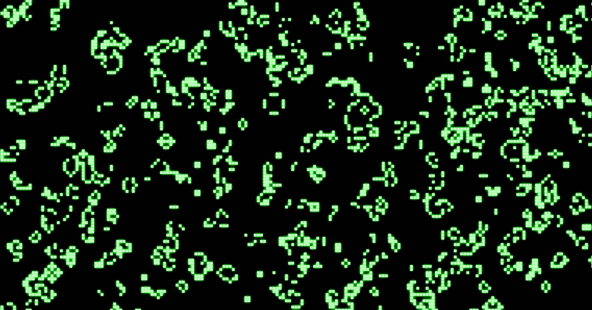
Let’s try implementing a more involved cellular automaton, we’re going to implement Wireworld, a cellular automaton first proposed by Brian Silverman in 1987 and particularly suited to simulating electronic logic elements, or “gates”. Wireworld is Turing-complete, even, meaning that you could simulate a full computer system with it.

We need to make the following changes. Cells can now have four distinct states:

• Empty
• Electron head (drawn in blue)
• Electron tail (drawn in red)
• Conductor, a wire (drawn in yellow)

The rule set is as follows:

• Empty cells stay empty
• Electron heads become electron tails
• Electron tails become conductors
• Conductor become an electron head if exactly one or two of the neighbouring cells are electron heads, otherwise remains conductor

The neighborhood again includes diagonal cells, but we’re not going to wrap around the grid. The implemented example looks as follows (press p to pause the simulation so you can draw freely — you might need to click in the iframe first to give it focus):

Finishing up

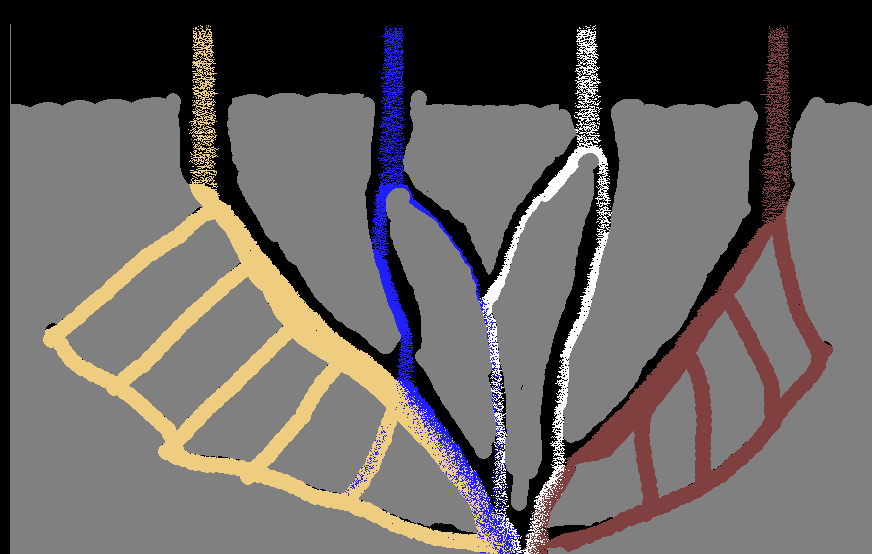
Cellular automata are very versatile indeed. As a final example, let us consider Langton’s Ant. This can be modelled as a discrete agent walking over a grid, but as the Wikipedia page mentions, it’s possible to formulate the behavior by means of a cellular automaton as well. Our state now encodes:

• Whether a cell is white or black
• Whether a cell contains an ant or not. If it contains an an, the numbers 1 to 4 indicate the direction of the ant

The rule set is as follows:

• The next cell’s color is equal to the current one, except if the ant is here, in which case we flip the color
• If the ant is on a cell, first figure out the new direction of the ant
• If the current cell’s color is black, turn 90 degrees left
• If it’s white, turn 90 degrees right
• The ant is removed from the next cell
• The ant is place on the next cell matching the new direction of the ant

In fact, we don’t even have to define a neighborhood here, except for knowing to which new cell to move our ant. This simple rule set leads to a beautiful pattern over time (this cellular automaton runs on its own, no way to scribble over it here):

That’s enough for the first part in this series. In the next part, we’ll use the building blocks we’ve constructed and explored so far, and start taking a look at using cellular automata to simulate water, sand, lava, and so on, as is done in several games.